LIDS: ultradian sleep-cycle dynamics from actigraphy

Sleep isn’t uniform from lights-out to wake-up: limb movement during sleep rises and falls in ~60-110 minute cycles that track the alternation between REM and non-REM sleep. Locomotor Inactivity During Sleep (LIDS) is a way to recover that ultradian structure from ordinary wrist/ankle actigraphy, without polysomnography – turning raw movement counts into an “inactivity” signal, then fitting a cosine to it to estimate cycle length, amplitude, and how inactivity trends over the course of the night.

zeitR’s LIDS module ports two papers:

Winnebeck, Fischer, Leise & Roenneberg (2018), Current Biology – the original method (adults/adolescents): the 100/(1+x) transform, moving-average smoothing, a plain cosine fit, and the Munich Rhythmicity Index (MRI) for period selection.
Hammad, Schoch, Engelmann, Spock, Kurth & Winnebeck (2026), SLEEP – an infant-tuned extension: Gaussian smoothing, a sloped cosine (adding a linear trend term to capture the well-documented overnight decline in inactivity), and a period scan tuned for shorter (~60 min) cycles.

This module has not yet been validated against pyActigraphy’s LIDS class or an external reference dataset – see ?compute_lids and ?fit_lids for exactly what’s ported from which paper, and treat results as exploratory until a parity check is run.

The pipeline in one call: `compute_lids()`

For a zeitr_result from run_pipeline() or run_pipeline_native(), compute_lids() does everything: extracts sleep bouts, transforms and fits each one, and returns a tibble with one row per bout.

FILE <- system.file("extdata", "input1.txt", package = "zeitR")
TZ   <- "America/Sao_Paulo"

result <- run_pipeline_native(FILE, tz = TZ, quiet = TRUE)
#> ℹ Reading input1.txt ...
#> ✔ [input1] Done. 52 main night(s), 0 secondary episode(s).

lids_bouts <- compute_lids(result, duration_range = c(3, 12))
lids_bouts
#> # A tibble: 36 × 14
#>    participant_id bout_id bout_start          bout_end            duration_h
#>    <chr>            <int> <dttm>              <dttm>                   <dbl>
#>  1 input1               1 2021-05-31 01:28:15 2021-05-31 06:09:15       4.68
#>  2 input1               2 2021-06-02 00:25:15 2021-06-02 06:01:15       5.6 
#>  3 input1               3 2021-06-02 23:42:15 2021-06-03 06:22:15       6.67
#>  4 input1               4 2021-06-04 00:01:54 2021-06-04 03:58:54       3.95
#>  5 input1               5 2021-06-04 23:45:54 2021-06-05 04:32:54       4.78
#>  6 input1               6 2021-06-06 00:41:54 2021-06-06 06:00:54       5.32
#>  7 input1               7 2021-06-07 00:13:54 2021-06-07 06:04:54       5.85
#>  8 input1               8 2021-06-08 01:53:54 2021-06-08 05:35:54       3.7 
#>  9 input1               9 2021-06-08 23:53:54 2021-06-09 06:26:54       6.55
#> 10 input1              10 2021-06-10 00:34:54 2021-06-10 05:45:54       5.18
#> # ℹ 26 more rows
#> # ℹ 9 more variables: period_min <dbl>, amplitude <dbl>, offset <dbl>,
#> #   slope_per_60min <dbl>, phase_rad <dbl>, pearson_r <dbl>, p_value <dbl>,
#> #   mri <dbl>, passes_quality_filter <lgl>

Each row is one detected sleep bout (state == 1 runs from the pipeline output, by default – see Where bouts come from below), with:

Column	Meaning
`period_min`	Estimated ultradian cycle length (minutes)
`amplitude`	Oscillation amplitude (LIDS units)
`offset`	Inactivity level at bout start
`slope_per_60min`	Linear trend in inactivity across the bout
`phase_rad`	Phase at bout start (`0` = LIDS peak at onset)
`pearson_r`, `p_value`, `mri`	Fit quality and the Munich Rhythmicity Index
`passes_quality_filter`	`TRUE` if the bout clears the Winnebeck/Hammad quality bar

mean(lids_bouts$passes_quality_filter)
#> [1] 1
summary(lids_bouts$period_min[lids_bouts$passes_quality_filter])
#>    Min. 1st Qu.  Median    Mean 3rd Qu.    Max. 
#>   36.00   51.50  101.00   98.94  123.50  180.00

Under the hood: a clean synthetic example

Because a real recording’s LIDS fit is noisy, it helps to see the method on a signal built to have a known answer first: a 60-minute sloped cosine with a little noise, the kind of ultradian cycle Hammad et al. (2026) report in infants.

set.seed(1)
t    <- seq(0, 300, by = 1)                                 # 5 h, 1-min epochs
true_period <- 60
lids_clean  <- 85 + 15 * cos(2 * pi * t / true_period) -
  0.05 * t + rnorm(length(t), sd = 1.5)

if (has_ggplot2) {
  ggplot(data.frame(t = t, lids = lids_clean), aes(t, lids)) +
    geom_line(colour = "#4A3F6B") +
    labs(x = "Minutes since bout onset", y = "LIDS",
         title = "Synthetic LIDS profile (period = 60 min)") +
    theme_minimal(base_size = 12)
}

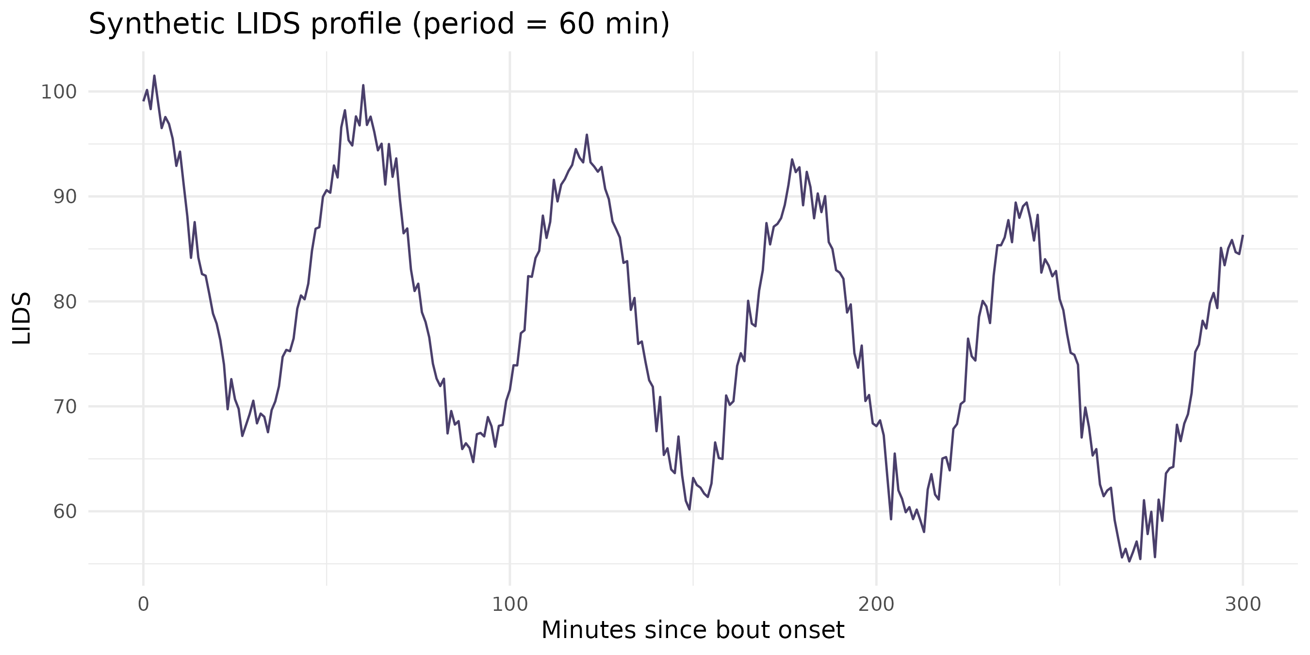
fit_lids() recovers the period, amplitude, and slope directly from this profile:

fit <- fit_lids(lids_clean, period_range = c(30, 120), period_step = 1)
fit[c("period_min", "amplitude", "offset", "slope_per_60min", "pearson_r", "mri")]
#> $period_min
#> [1] 60
#> 
#> $amplitude
#> [1] 15.13642
#> 
#> $offset
#> [1] 85.12597
#> 
#> $slope_per_60min
#> [1] -3.028703
#> 
#> $pearson_r
#> [1] 0.9923784
#> 
#> $mri
#> [1] 30.0421

From activity to LIDS: `lids_transform()`

In practice you start from raw activity counts, not a pre-built LIDS profile. lids_transform() applies the 100/(1+x) non-linear transform and smooths the result – higher activity means lower inactivity, and smoothing suppresses epoch-to-epoch noise so the underlying oscillation is fittable.

set.seed(2)
activity <- pmax(0, 30 + 20 * sin(2 * pi * t / true_period) + rnorm(length(t), sd = 8))

lids_gaussian <- lids_transform(activity, method = "gaussian")   # Hammad et al. 2026
lids_mva      <- lids_transform(activity, method = "mva")        # Winnebeck et al. 2018

if (has_ggplot2) {
  df <- data.frame(
    t = rep(t, 2),
    lids = c(lids_gaussian, lids_mva),
    method = rep(c("gaussian", "mva"), each = length(t))
  )
  ggplot(df, aes(t, lids, colour = method)) +
    geom_line() +
    scale_colour_manual(values = c(gaussian = "#C25E2A", mva = "#4A3F6B")) +
    labs(x = "Minutes since bout onset", y = "LIDS", colour = "Smoothing",
         title = "Gaussian (Hammad 2026) vs. moving-average (Winnebeck 2018) smoothing") +
    theme_minimal(base_size = 12)
}

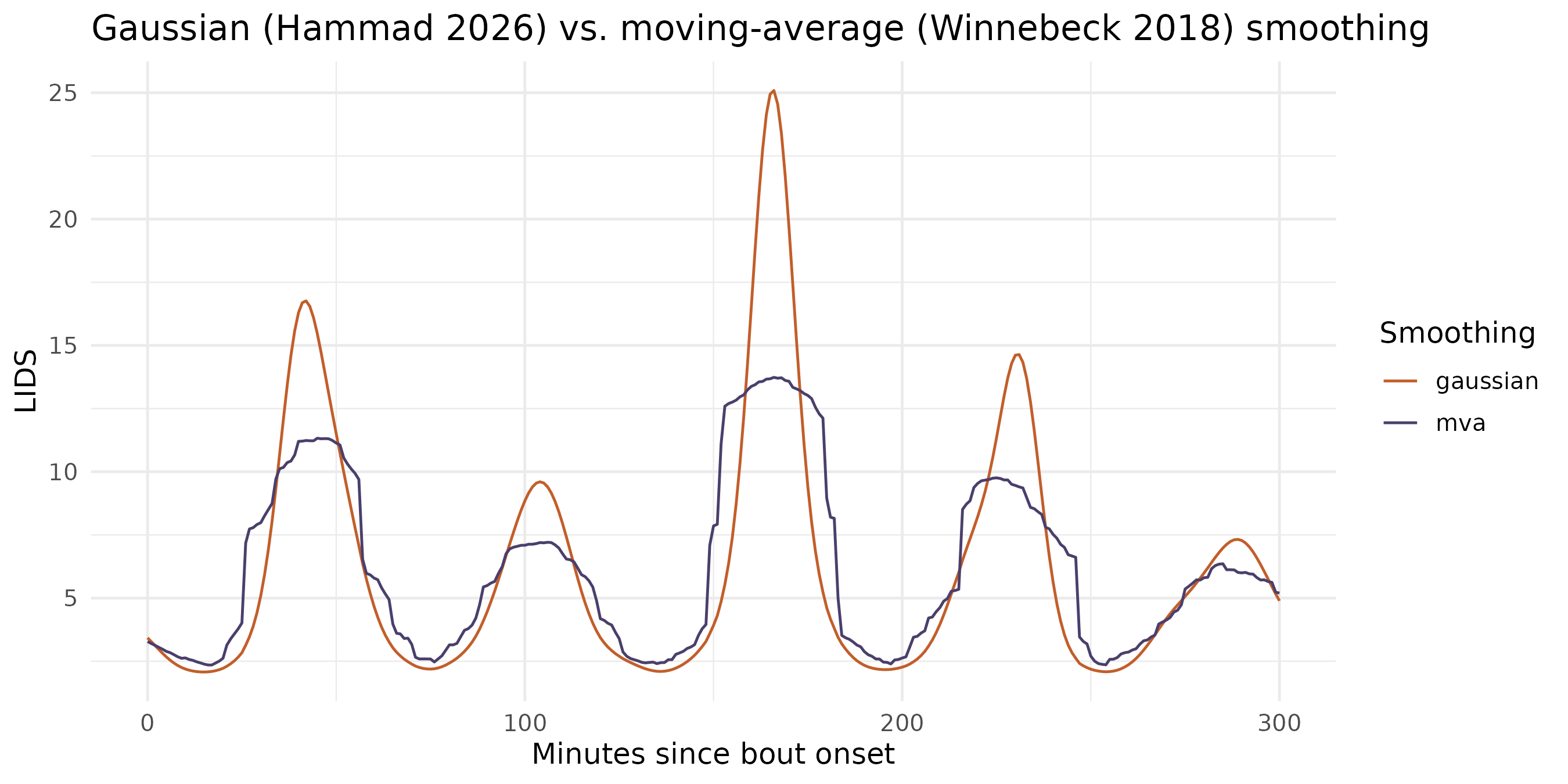
Both methods track the same underlying oscillation; Gaussian smoothing (the default) is slightly less aggressive at suppressing sharp transients, which matters more for the shorter cycles and higher amplitudes seen in infants than for adults.

Where bouts come from

compute_lids()’s bout_source argument controls how sleep bouts are identified:

"state" (used automatically above, since result$data already has a state column) – contiguous state == 1 runs from an existing zeitR pipeline result. This is almost always what you want if you’ve already run run_pipeline() or run_pipeline_native().
"roenneberg" – ignores any state column and runs the standalone detect_lids_bouts() relative- immobility detector directly on raw activity, reproducing Winnebeck/Hammad’s own bout-detection method rather than zeitR’s Crespo/Vallim pipelines. Use this for activity data you haven’t run through either pipeline.
"auto" (the default) picks "state" if available, "roenneberg" otherwise.

bouts <- detect_lids_bouts(
  result$data$datetime, result$data$activity,
  duration_range = c(3, 12)
)
nrow(bouts)
#> [1] 39
head(bouts)
#> # A tibble: 6 × 5
#>   bout_id bout_start          bout_end            duration_h n_epochs
#>     <int> <dttm>              <dttm>                   <dbl>    <int>
#> 1       1 2021-05-27 23:40:15 2021-05-28 07:03:15       7.38      444
#> 2       2 2021-05-28 23:28:15 2021-05-29 07:30:15       8.03      483
#> 3       3 2021-05-30 22:17:15 2021-05-31 08:03:15       9.77      587
#> 4       4 2021-05-31 23:24:15 2021-06-01 07:10:15       7.77      467
#> 5       5 2021-06-02 23:36:15 2021-06-03 07:49:15       8.22      494
#> 6       6 2021-06-03 22:43:54 2021-06-04 07:46:54       9.05      538

Quality filtering

Not every bout yields a clean ultradian fit – a device removed mid-sleep, an unusually short or fragmented bout, or genuine absence of rhythmicity can all produce a poor fit. compute_lids() flags (rather than silently drops) bouts failing the Winnebeck/Hammad quality bar:

table(lids_bouts$passes_quality_filter)
#> 
#> TRUE 
#>   36

lids_bouts[!lids_bouts$passes_quality_filter,
           c("bout_id", "duration_h", "pearson_r", "p_value", "offset")]
#> # A tibble: 0 × 5
#> # ℹ 5 variables: bout_id <int>, duration_h <dbl>, pearson_r <dbl>,
#> #   p_value <dbl>, offset <dbl>

Adjust the thresholds directly if the defaults (min_r = 0.4, max_p = 0.05, offset_bounds = c(1, 99)) don’t suit your data:

compute_lids(result, min_r = 0.3, max_p = 0.1)

Study-level summaries

For a whole cohort, study_lids_metrics() reduces each participant’s quality-filtered bouts to one row – median and IQR period, amplitude, offset, and slope – ready for syncR::sync() the same way study_sleep_metrics() and study_summary() already are.

results <- run_pipeline_native_batch("recordings/", tz = "America/Sao_Paulo")
study_lids_metrics(results, min_bouts = 3)

Next steps

?compute_lids – full argument reference, bout_source details, and the quality-filter rationale
?fit_lids, ?lids_transform – the underlying cosine fit and smoothing, if you need to build a custom pipeline around them
?detect_lids_bouts – the standalone bout detector, including what differs from the Winnebeck/Hammad notebook it was ported from
Winnebeck et al. (2018), Current Biology 28(1), 49-59.e5, https://doi.org/10.1016/j.cub.2017.11.063
Hammad et al. (2026), SLEEP – infant ultradian cycle lengthening, https://zenodo.org/records/18199381

The pipeline in one call: compute_lids()